True Peak Detection

Russell McClellan

In the last few years, a number of different countries have passed laws regulating the loudness of audio in television and other broadcast mediums. Surprisingly, loudness is a difficult concept to capture with a simple technical specification. Current regulations set limits for a number of different audio metrics, including overall loudness, maximum short-term loudness, and the true peak level of a signal.

What are true peaks?

To understand how true peaks differ from sample peaks, we have to go back to the basis of digital audio: the Sampling Theorem. This theorem states that for every sampled digital signal, there is only one correct way of reconstructing a band-limited analog signal into a digital one such that the analog signal passes through each digital sample. Digital-to-analog converters try to approximate this correct analog waveform as closely as possible. For more details on this fascinating theorem, we recommend this video from xiph.org.

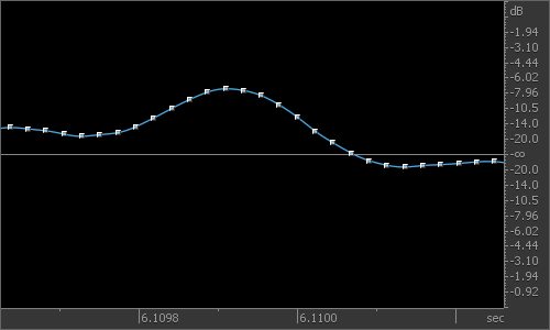
Some audio editors are able to display the digital samples and an approximation of the corresponding analog waveform. In iZotope RX, both of these signals appear when you zoom far enough in. The blue line represents the analog signal, while the white squares are the digital samples.

In RX, you can click and drag on an individual sample to change it and see how the analog signal reacts. For example, if you move a single sample very far, we can see that a large amount of ripple appears in the analog signal around that sample.

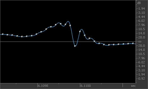
It’s clear that the analog signal’s peak is quite a bit higher than the highest digital sample. The highest point the analog signal reaches is called the true peak while the highest digital sample is called the sample peak. Since a digital signal has to be converted to an analog signal to be heard, the true peak is a much more sensible metric for the peak level of a waveform.

It turns out that for real audio signals, quite often the true peak is significantly higher than the sample peak, so it’s important to measure carefully.

How are true peaks detected?

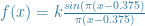
BS.1770, the international standards document used as the base for regional loudness specifications, gives a suggested algorithm to detect the true peak level of a digital signal. This algorithm is a relatively simple one: first, upsample the signal to four times its original sampling rate, and then take the digital peak of the new, upsampled signal. We can perform this algorithm manually in RX: first, open the “Resample” module and select a sample rate four times the original rate, then open the waveform statistics window and check the sample peak level. Here’s what the test signal above looks like after it has been upsampled to four times its original rate:

As you can see, after upsampling, the true peak level is now very close to the sample peak.

Of course, the RX waveform statistics window already provides the true peak level, so you don’t have to perform these steps by hand.

While this algorithm is quite good, there are two major ways that errors can occur. First, no upsampling algorithm can ever be perfect, so either overshoots or undershoots can occur during the upsampling process. This problem can be helped by using a high-quality upsampling algorithm. Second, the true peak may still be between samples even after the upsampling happens. This problem can be ameliorated by upsampling at a higher ratio.

How can we measure the quality of a true peak meter?

While most true peak meters follow the same basic algorithm as the one described in BS.1770, they can vary significantly in two dimensions: the quality of the upsampling algorithm, and also in the ratio of upsampling. BS.1770 includes a description of a simple upsampling algorithm, but many true peak meters actually perform more accurate upsampling than required by the specification. Also, many meters upsample by more than the required four times. This means that true peak meters can vary significantly in the accuracy of their output.

How can the quality of a meter be measured? One way is to create a synthetic signal that is difficult to meter accurately, but has a mathematically known true peak. This way, we can compare the meter’s reported true peak to the true peak we calculated ahead of time, and any difference can be attributed to meter error.

Testing meters with single impulses

One simple signal with a known true peak is a digital impulse, a signal with all samples at zero except for a single sample at a non-zero value. We can see the analog waveform this creates by looking at it in RX:

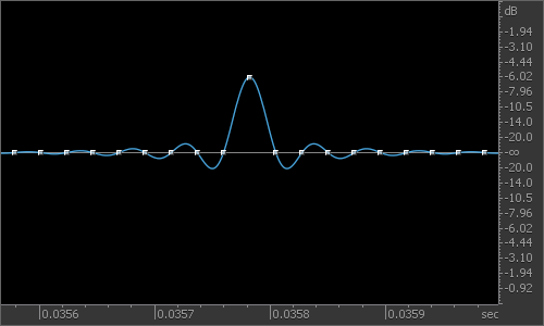
It turns out that the analog waveform for a digital impulse is a well studied function called the sinc function and has a simple mathematical expression: 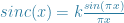. Also, the true peak is the same as the sample peak at . This isn’t an incredibly useful signal for testing true peak meters, since even a bad true peak meter that only looks at the sample peak without upsampling will get the correct answer.

However, knowing the mathematical expression for the analog signal allows us to shift it in time to create a more interesting signal. Consider a signal the same function with a time offset of a fraction of a sample, say , i.e., . This signal should still have a true peak of , since time shifting an analog signal will not change its analog peak. However, the sample peak will be lower, since the true peak no longer sits exactly on a digital sample.

We can use Python, NumPy, and scikits.audiolab to create a wave file with this shifted sinc signal:

import numpy as np
from scikits.audiolab import Format, Sndfile

def save_file(arr, filename):
format = Format('wav')
f = Sndfile(filename, 'w', format, 1, 48000)
f.write_frames(arr)
f.close()

def shifted_sinc(x):
k = 0.5
offset = 0.375
return (k * np.sin(np.pi * (x - offset)) /
(np.pi  * (x - offset)))

length = 48000
out = shifted_sinc(np.arange(length, dtype='float') -
length / 2)
save_file(out, 'shifted_sinc.wav')

Then, we can open it in RX to see the digital samples and analog waveform:

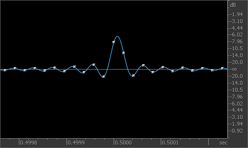
As we can see, the analog waveform is the same, only shifted in time. However, now the sample peak is a few decibels lower than the true peak. We set , so the true peak is or dB. The sample peak is the sample immediately before the true peak, which using our formula above is or around dB, a difference of over two decibels from the true peak!

Since we know the exact true peak level of this signal, we can use it as a test of a true peak meter. It’s fairly difficult to measure, because a sinc function contains information at all frequencies up to the Nyquist frequency, making it difficult to upsample accurately. Also, the peak is located at a fraction of , so even perfect upsampling by four would not catch the true peak. You can download this shifted sinc test file here.

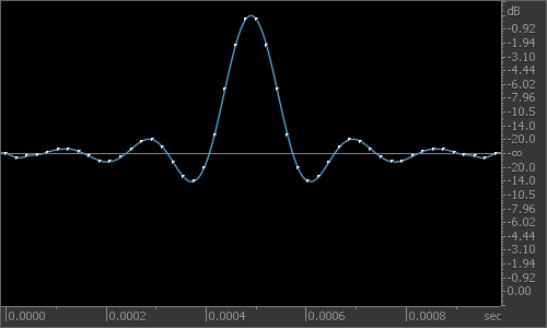
Testing Overshoot: Sine Sweeps

Another good test for true peak meters is a sampled sine sweep at a known amplitude. The true peak of this waveform will just be the amplitude of the sine sweep, but many meters will report a higher true peak because of errors in the upsampling algorithm. Like the sinc function, the sine sweep is difficult to upsample accurately because it has information at all frequencies. We can generate a sine sweep with the following NumPy code:

import numpy as np
from scikits.audiolab import Format, Sndfile

def save_file(arr, filename):
format = Format('wav')
f = Sndfile(filename, 'w', format, 1, 48000)
f.write_frames(arr)
f.close()

def sine_sweep(begin_freq, end_freq, length, fs, scale):
# The instantaneous frequency at each sample
freqs = np.linspace(begin_freq, end_freq, length)
freqs /= fs

# The angular frequency of the sweep at each sample
omegas = freqs / 2 * np.pi

# The phase of the sweep at each sample
phases = np.cumsum(omegas)

# Create a fade in and out to avoid artifacts at
# the beginning and the end.
fade_length = length / 8
fade_in = np.linspace(0, 1, fade_length)
fade_out = np.linspace(1, 0, fade_length)
fade = np.ones(length)
fade[:fade_length] = fade_in
fade[length - fade_length:] = fade_out
return fade * scale * np.sin(phases)

sweep = sine_sweep(200, 23000, 48000, 48000, 0.5)
save_file(sweep, 'sine_sweep.wav')

You can download the sine sweep file here.

How good is the example algorithm specified by BS.1770?

Now that we have a few techniques for measuring the quality of true peak detection algorithms, let’s put these to work in evaluating the example algorithm provided by BS.1770.

The upsampling algorithm is a simple one, based on upsampling by four, interpolating with a specific kernel. For more background information on upsampling, please see this reference. The coefficients of the kernel are given in the BS.1770 specification, and looks like this:

If we save this kernel as a wave file we can use RX’s Spectrum Analyzer to visualize the frequency response of this kernel:

Here, the cutoff frequency is a quarter of the sampling rate, or 6 kHz. The ideal filter would be perfectly flat below this frequency, and then drop immediately down to dB above it. Real world resampling filters have to make tradeoffs and cannot achieve this.

As we can see, there is a fairly significant amount of ripple in the passband (below roughly 5 kHz), which may indicate that the detector will overshoot at certain frequencies. Indeed, applying this detector to our sine sweep test signal, which has a true peak level of dB, results in a measured value of dB, an error of dB.

Also, the kernel is not very steep at our cutoff frequency. This indicates that for signals with a lot of high-frequency content, such as our sinc test signal, the filter may significantly undershoot. Indeed, for our shifted sinc test file, which also has a true peak of dB, the BS.1770 detector results in a measured value of dB, an error of dB. So, even compliant meters can have fairly significant errors in their true peak detection.

Extra credit: How high can true peaks get?

We’ve now seen several signals that have true peaks higher than their sample peaks, even by more than a decibel. Is there any limit to how much higher the true peaks can be than the sample peak? This is an interesting question because if there were some limit than we would have a worst case bound of how much error any given true peak meter could have.

Unfortunately for meters, it turns out that there is actually no limit to the difference between sample peaks and true peaks.

Plan of the Proof

To show that true peaks can become arbitrarily high, we’ll explore a pathological waveform where we can make the true peak as high as we want, by adding more samples. This particular example was discovered by iZotope colleague Alex Lukin, and the rigorous proof that it had an unboundedly high true peak was found by Aaron Wishnick.

The pathological waveform we are interested in is a series of alternations between and , followed by silence. We’ll show that by adding more alternations, we can make the true peak as high as we want to.

We can start to get a feel for this waveform by manually dragging samples around in RX. Here’s what it looks like after three alternations of and :

As you can see, one true peak is already higher than the sample peak of , and it’s exactly halfway between samples. Using RX’s waveform stats window, we can see that after three alternations the true peak is dB, while the sample peak is or dB. It turns out that by adding more alternations of and , we can make the true peak even higher. Here’s what it looks like with ten alternations:

Using waveform stats, we see that the true peak is dB, while the sample peak is the same at dB.

In order to prove that we really can make the true peak as high as we want, we’ll have to dig into some of the math.

Detailed Proof

For convenience, let’s call the time of the last sample time , so that the alternations of and extend back into negative time. Also for convenience, let’s assume our sampling rate is (this will make the math a bit easier). Judging from RX, this will put the true peak at time , half way between the last and the first .

So, we need to find an equation to tell us the value of the analog waveform at time . For this, we can use the Shannon interpolation formula:

Where is our sampled signal at time , is the number of alternations and is the analog waveform at time . Since we are interested in , our equation becomes

We know from trigonometry that is positive if is even, or negative if is odd. We can express this as . So our equation becomes

Now, we plug in the fact that our signal consists of alternations between and , ending at at time 0. Note that when is even, and when is odd, since it alternates every sample. We can express this as . So, our equation simplifies to

Now, note the two terms cancel:

This is a formula for the analog level at time that only depends on the number of alternations, .

We can plot this series using Wolfram Alpha, and note that the sum diverges. We can also recognize this as a general harmonic series, which all diverge.

Knowing that the series diverges means that the more terms we add the more alternations of and , the higher the true peak will be. There is no limit to how high we can make the true peak, if we have enough alternations of and . However, since the signal is either , , or at all samples, the sample peak is always . So, knowing the sample peak doesn’t tell you much about the true peak, at least for these pathological signals.